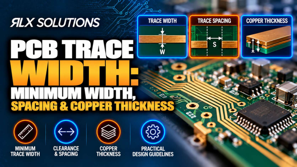
PCB trace width and spacing cannot be specified independently of copper thickness. A geometry that is practical in 1 oz copper may need wider traces and gaps in 2 oz copper because etching removes copper laterally as well as vertically. RLX Solutions, a contract electronics manufacturer in Concord, Ontario, reviews these relationships against the complete stackup before fabrication.
PCB trace width starts with electrical requirements, then meets fabrication limits
A PCB trace is the patterned copper conductor connecting two electrical points on a printed circuit board. Its required width comes from electrical behaviour first: current, acceptable temperature rise, voltage drop, impedance and signal geometry can all establish a minimum.
Fabrication then imposes another constraint. The trace has to survive imaging, developing and etching while remaining inside the required dimensional window. That makes the final design rule a combination of electrical need and manufacturing feasibility.
This distinction matters because “minimum trace width” can mean two different things:
- Electrical minimum: the width required for current, resistance, temperature or impedance.
- Fabrication minimum: the narrowest feature that can be produced reliably for the selected copper thickness and stackup.
Your layout must satisfy both. A trace that passes a current calculation but falls below the fabrication limit is not manufacturable as drawn. A trace that is easy to fabricate but too narrow electrically may overheat or create unacceptable voltage drop.
For bare PCB fabrication, trace width and trace spacing are commonly expressed together. A 3 mil / 3 mil rule means a minimum 3 mil trace with a minimum 3 mil copper-to-copper gap.
Start with the actual copper on each layer
Do not assign one trace-width rule to the entire board unless the stackup supports it.
Outer and inner layers can have different copper weights. They also experience different fabrication conditions. A power layer using heavier copper may therefore need different design rules from a signal layer using thinner copper.
Copper weight is a convenient manufacturing description of copper thickness. As copper gets thicker, its cross-sectional area increases. For the same trace width, that generally reduces conductor resistance and improves current-carrying capability. The trade-off appears during etching, where thicker copper makes fine geometry harder to preserve.
Copper thickness changes what the etching process can reproduce
The reason heavier copper tends to need wider traces and spaces is physical. PCB fabrication does not remove unwanted copper only straight downward.
During etching, chemistry also attacks the sides of the copper feature. This lateral removal is commonly associated with undercut. As copper thickness increases, more etching is required to clear unwanted material, which makes narrow conductors and small gaps harder to control.
That creates two opposing design pressures.
For power distribution, thicker copper is attractive because it provides more conductor cross-section. For dense routing, thinner copper makes narrow traces and spaces easier to manufacture.
Consider a simple two-layer board:
| Design factor | Board A | Board B |
|---|---|---|
| Layer count | 2 | 2 |
| Outer copper | 1 oz | 2 oz |
| Proposed trace/space | 3 mil / 3 mil | 3 mil / 3 mil |
| Fabrication geometry | Within a 3/3 mil 1 oz process | Too aggressive for a 6/6 mil 2 oz process |
| Practical response | Keep 3/3 mil where density requires it | Increase geometry to at least 6/6 mil or reconsider copper weight |
The boards have the same layer count and can even have identical outlines and drill files. They are not equivalent fabrication jobs.
For 2-layer, 1 oz construction, 3 mil / 3 mil trace and spacing can be produced within the fabrication range. With 2 oz copper on a two-layer board, the corresponding geometry is 6 mil / 6 mil. The additional copper helps the electrical cross-section but changes the etching problem.
This is why increasing copper weight after layout is complete can trigger rerouting. It is not simply a material substitution.
Minimum PCB trace width and spacing are stackup decisions
Trace and space rules should be assigned after the layer structure and copper weights are known. On a multilayer PCB, the same nominal line width can appear on several layers without those layers being physically equivalent.
For example, consider a four-layer, 1 oz design with 3 mil traces on Layer 1. A designer may need that geometry to escape a dense component area before transitioning through vias to a less congested layer. A 3 mil / 3 mil outer-layer geometry is within the fabrication range for this construction.
Now change the project to a six-layer board while retaining 3 mil / 3 mil routing. That geometry remains possible, but the stackup deserves engineering review because registration, dielectric construction, copper distribution and other features now interact across more layers.
Fine-line routing pushes this further. Selected 2 mil / 2 mil sections can be considered for a high-density interconnect (HDI) design with an engineered stackup. That should not become a global design rule merely because one local escape region needs it.
A better layout strategy is to keep aggressive geometry local. Use fine lines where component escape or routing density demands them, then widen the conductors once they leave the constrained region.
That reduces manufacturing pressure without giving up the density that forced the fine-line section in the first place.
Trace spacing has more than one job
Copper spacing is the edge-to-edge distance between adjacent copper features. Fabrication sets one lower boundary, but electrical requirements may force a much larger gap.
The etching process needs enough separation to remove copper cleanly between conductors. At the same time, voltage difference, insulation requirements, controlled impedance geometry and electromagnetic coupling can determine spacing independently of the fabrication minimum.
That means a manufacturer’s minimum spacing is not an electrical design recommendation.
A 3 mil fabrication capability does not mean two conductors carrying a particular voltage should be separated by 3 mil. It means the manufacturing process can resolve that geometry under the specified construction. Electrical clearance and creepage requirements still have to be established from the product’s operating conditions and applicable design requirements.
Copper near the board edge needs its own rule
Routing density sometimes pushes copper toward the finished outline, especially around connectors, mounting hardware and compact mechanical envelopes.
Copper-to-edge clearance needs to account for board profiling and positional tolerances. A minimum 0.3 mm copper-to-edge clearance provides a concrete fabrication constraint for layout.
This is easy to miss because the nearest object is not another trace. A design-rule check focused only on trace-to-trace spacing can therefore pass while a copper pour or conductor remains too close to the routed edge.
Include copper-to-edge clearance as a separate board-level rule.
Use heavier copper where the current needs it, not automatically everywhere
Increasing copper weight is one way to increase conductor cross-section, but it is not the only one. Trace width also contributes directly.
For a rectangular conductor, cross-sectional area is driven by width multiplied by copper thickness. If routing space exists, widening a power trace can increase copper area without forcing every feature on that layer into a heavier-copper fabrication process.
This matters on mixed-density boards.
Imagine a board with a dense digital region and several higher-current power paths. Moving an entire two-layer design from 1 oz to 2 oz copper changes the fabrication geometry available across the board. If the dense region needs 3 mil / 3 mil routing, the heavier copper creates a conflict because 2 oz construction calls for 6 mil / 6 mil geometry.
One possible design response is to retain 1 oz copper and allocate more width to the power conductors. Another is to redesign the routing around 2 oz copper and accept the larger minimum geometry. The correct path comes from the electrical calculations and available board area, not from copper weight alone.
For applications that genuinely require substantial conductor cross-section, outer copper can extend through 3 oz as a standard option, with 4 to 6 oz outer copper considered for heavy-copper builds. Inner copper is available at 0.5, 1 and 2 oz, with up to 3 oz considered for heavy-copper construction.
As copper becomes heavier, confirm the actual geometry rather than assuming ordinary fine-line rules still apply.
Controlled impedance can override your preferred trace width
A controlled-impedance trace is a transmission line whose geometry and surrounding dielectric structure are designed to produce a specified impedance. Width is therefore part of an electrical system, not an isolated routing choice.
Trace width interacts with factors such as:
- copper thickness
- dielectric thickness
- dielectric properties
- reference-plane relationship
- spacing to coupled traces
- final stackup construction
This creates a common conflict. The layout engineer may choose a trace width based on routing density, while the impedance model requires a different width once the actual laminate and dielectric thicknesses are established.
Suppose a six-layer design routes a controlled signal on Layer 1 referenced to Layer 2. You cannot lock the Layer 1 width in isolation and treat the dielectric between Layers 1 and 2 as an interchangeable fabrication detail. Changing that dielectric changes the transmission-line geometry.
The stackup and impedance target should therefore travel with the fabrication data.
Controlled impedance can be produced to ±10%, with time-domain reflectometry (TDR) verification on a coupon and a test report supplied with the order. Requirements tighter than ±5% need project-specific review.
The larger lesson is useful even for non-controlled nets: copper geometry belongs to the stackup.
Fine traces often implicate vias, pads and solder mask next
Shrinking a trace solves only one part of a dense routing problem. Once routing density forces 3 mil or 2 mil conductors, the design often encounters restrictions elsewhere.
A fine-pitch ball grid array (BGA), for example, may not have enough routing channels for conventional through vias and wide traces. The escape architecture can then move toward laser-drilled microvias, blind vias or via-in-pad.
Laser-drilled microvias can reach 0.10 mm, with stacked and staggered configurations considered for HDI structures. Via-in-pad can use resin fill, copper capping and planarization on multilayer construction. Blind vias on 4+ layer stackups require sequential lamination, so changing the via architecture changes the manufacturing sequence itself.
Consider a hypothetical six-layer board with a dense component requiring a Layer 1 to Layer 2 microvia escape. If Layer 1 uses a 2 mil / 2 mil section to leave the pad field, widening to 4 or 5 mil once the trace clears that region reduces the amount of fine-line geometry without changing the component placement.
If that via sits directly in a component pad, fill and cap become part of the pad construction. The routing decision has now affected drilling, plating, filling, planarization and lamination.
Solder mask can become another limiting geometry. A minimum 0.08 mm mask dam is available between pads, with 0.05 mm per-side mask expansion as the default. Dense copper routing should therefore be reviewed together with pad and mask geometry rather than as a trace-only exercise.
Do not solve trace width without checking the drill structure
Routing density and via density are closely connected. Narrowing traces can create another routing channel, but the via architecture still consumes pad and annular-ring area.
Mechanical plated through-holes can use drills down to 0.15 mm. The minimum annular ring is 0.075 mm on inner layers and 0.1 mm on outer layers. Those dimensions affect how much routing space remains between via structures.
Board thickness matters as well because plated-hole geometry has an aspect ratio. The standard maximum aspect ratio is 10:1, with 12:1 considered where the construction supports it.
This can produce a design that appears spacious in two-dimensional CAD but is difficult in the actual manufacturing sequence.
For example, a 1.6 mm-thick board with very small mechanical holes cannot be judged solely by the visible drill diameter. The hole depth relative to diameter affects drilling and plating. If the design then replaces those structures with blind or laser-drilled vias to recover routing space, lamination and via processing change too.
Trace width, drill architecture and stackup should be resolved together before routing is treated as final.
Board A vs Board B: same layer count, very different fabrication burden
| Decision factor | Board A | Board B |
|---|---|---|
| Layers | 6 | 6 |
| Main trace/space | 3 mil / 3 mil | 3 mil / 3 mil |
| Fine-line region | None | 2 mil / 2 mil selected section |
| Via architecture | Through-hole PTH | Layer 1 to 2 microvias plus via-in-pad |
| Fine-line purpose | Not required | Dense component escape |
| Additional process interaction | Conventional multilayer routing | Laser drilling, filling/capping where specified, tighter local imaging |
| Engineering focus | Stackup, registration, drilling | Stackup plus HDI build sequence and fine-line region |
Both boards say “six layers” on a quote request. Board B carries more manufacturing dependencies.
The important cost mechanism is not simply that its traces are narrower. The 2 mil section exists because the routing architecture is denser, and that density may trigger laser drilling, filled and capped vias, additional process control and an engineered stackup.
This is why reducing every conductor by a mil to make routing easier in CAD can have the opposite effect on manufacturing. A local layout problem can become a board-wide fabrication constraint.
Set PCB design rules by layer and function
A single global minimum is convenient but can hide the decisions that matter. Build design rules around the physical construction and the function of each conductor.
- Establish the stackup and copper weight. Identify outer and inner copper separately.
- Calculate electrical requirements. Size power conductors for current, resistance, voltage drop and thermal behaviour.
- Define impedance geometry. Resolve trace width against dielectric construction and reference planes.
- Identify density bottlenecks. Determine where ordinary routing geometry cannot escape the component field.
- Apply fine-line rules locally. Do not make a 2 mil escape requirement the default for an entire board.
- Check via architecture. Mechanical, blind, buried and laser-drilled vias change routing space and manufacturing sequence.
- Check solder mask and board edges. Copper spacing is not the only geometric constraint.
- Release the stackup with the fabrication data. Include impedance targets where controlled impedance is required.
This approach preserves routing freedom where you need it while keeping the rest of the circuit board inside less demanding geometry.
Send trace rules as part of the manufacturing definition
Gerber RS-274X, ODB++, IPC-2581 and NC drill data can define the physical bare board, but dense or impedance-controlled designs benefit from explicit stackup and impedance documentation as well.
Do not leave the fabricator to infer whether a narrow conductor is intentional, whether copper weight can change, or whether a particular width belongs to an impedance-controlled net.
If you are preparing a board for prototype or production, RLX includes engineer-reviewed design for manufacturability (DFM) review on every quote. Send the manufacturing files, stackup and impedance targets so trace width, spacing, copper thickness, drilling and adjacent processes can be reviewed as one build.
FAQ
Is 3 mil trace and 3 mil spacing manufacturable?
Yes, for specified constructions. A 2-layer board with 1 oz copper can use 3 mil / 3 mil trace and spacing, as can a 4-layer board with 1 oz outer copper. Six-layer and higher constructions can also use 3 mil / 3 mil geometry with engineering review. Copper weight and stackup still need to be considered together.
Can a PCB use 2 mil traces?
Selected 2 mil / 2 mil sections can be considered for HDI fine-line construction with an engineered stackup. Treat that geometry as a local density tool rather than an automatic board-wide design rule. If 2 mil routing is required for component escape, the associated via structure, copper weight, solder mask and layer stack should be reviewed together.
How does 2 oz copper affect minimum trace spacing?
On a two-layer PCB, moving from 1 oz to 2 oz copper changes the stated trace-and-space geometry from 3 mil / 3 mil to 6 mil / 6 mil. Thicker copper requires more etching, which makes narrow conductors and gaps harder to reproduce. Changing copper weight late can therefore require routing changes.
Should power traces use 2 oz copper?
Copper weight should follow the electrical and layout requirements rather than a universal rule. Increasing thickness adds conductor cross-section, but increasing trace width does too. If a board needs dense 3 mil routing elsewhere, moving the entire layer to 2 oz can create a fabrication conflict that wider local power conductors may avoid.
What files should I provide for a trace-width review?
Provide the manufacturing data in Gerber RS-274X, ODB++ or IPC-2581 format with NC drill data. Include the stackup PDF and impedance targets when applicable. For an assembled-board quote, the BOM, pick-and-place or centroid file, and assembly drawing provide the additional information needed to review the complete build.
Does controlled impedance determine PCB trace width?
It can. Controlled-impedance width depends on the transmission-line geometry, including copper thickness, dielectric construction and the relationship to reference planes. That means an impedance trace should not be sized from routing density alone. The proposed stackup and impedance target should be resolved together before the geometry is considered final.