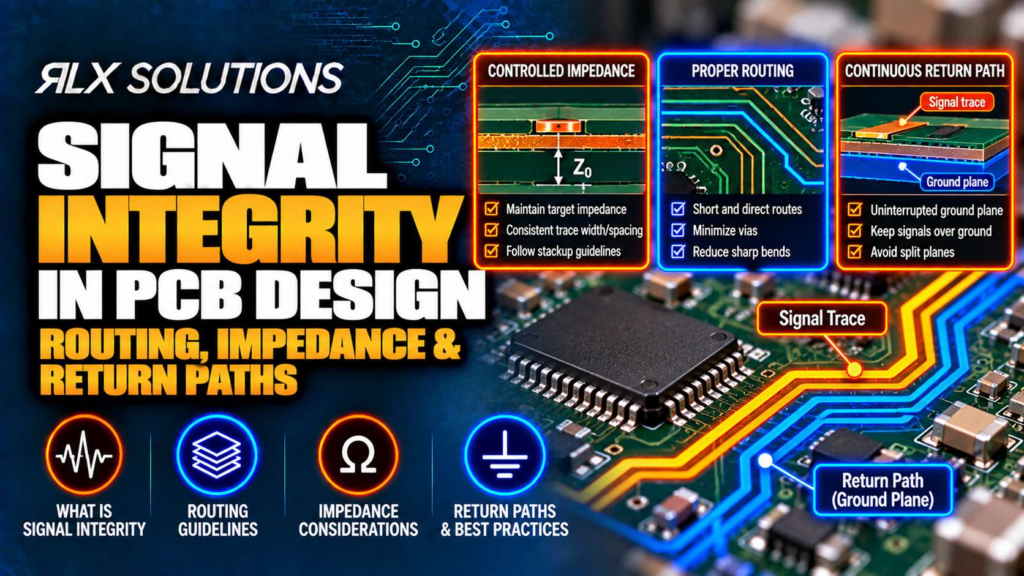
Signal integrity in PCB design depends on treating the trace and its return path as one electromagnetic structure. Controlled impedance, reference-plane continuity, via placement and stackup geometry all affect what reaches the receiver. RLX Solutions, a contract electronics manufacturer in Concord, Ontario, reviews these relationships before the circuit board moves into fabrication.
Signal integrity starts with the interconnect, not the schematic
A digital connection stops behaving like an ideal wire when its propagation delay becomes significant relative to the signal edge rate. At that point, the driver, PCB trace, vias, connectors, receiver and return path form a transmission system.
This distinction matters because clock frequency alone does not determine whether a net needs signal integrity treatment. A relatively low-frequency interface driven by a device with fast rise and fall times can produce reflections, ringing and crosstalk. The edge contains frequency content well above the fundamental switching rate.
Signal integrity is the preservation of a signal’s electrical shape and timing as it travels from transmitter to receiver. In PCB layout, that means controlling the physical structures that determine impedance, coupling and current return.
Three layout decisions dominate:
- Routing geometry: trace width, spacing, length and layer transitions.
- Impedance: the relationship among trace geometry, dielectric properties and reference planes.
- Return paths: the conductive path followed by the signal’s high-frequency return current.
These decisions are linked. Changing layers to improve routing density can change both impedance and the return-current path. Moving a trace farther from its reference plane can alter impedance while increasing its electromagnetic field area. Solving one variable in isolation can therefore create another problem.
Controlled impedance is a stackup property
Controlled impedance is not simply a trace-width instruction. It is the result of the complete transmission-line geometry.
For a surface microstrip, the important variables include conductor width and thickness, dielectric thickness to the reference plane, dielectric properties and the surrounding material. For an internal stripline, the relationship to reference planes above and below the trace also matters.
That is why specifying “50 Ω” in a fabrication note without defining or coordinating the stackup is incomplete. The fabricator has to convert the electrical target into manufacturable geometry.
A controlled-impedance PCB therefore connects two design domains:
| Design variable | Electrical consequence |
|---|---|
| Trace width | Changes characteristic impedance |
| Copper thickness | Changes the conductor geometry used in the impedance calculation |
| Dielectric thickness | Changes coupling between trace and reference plane |
| Dielectric properties | Change propagation and impedance behaviour |
| Reference-plane location | Affects impedance and return-current geometry |
| Differential spacing | Changes coupling within a differential pair |
| Fabrication variation | Produces variation around the intended impedance |
For boards requiring controlled impedance, fabrication can target ±10% impedance and verify the result by time-domain reflectometry (TDR) on a coupon. The test report then provides evidence that the manufactured transmission structure matches the specified impedance range.
A 50 Ω callout does not freeze the trace width
Consider a hypothetical 8-layer, 1.6 mm PCB. A designer routes a 50 Ω single-ended interface on Layer 1 over a Layer 2 ground plane.
Suppose the preliminary field-solver geometry calls for a 0.13 mm trace over a 0.10 mm dielectric. If the production stackup changes that dielectric separation to 0.14 mm, keeping the 0.13 mm trace does not automatically preserve 50 Ω.
The manufacturing question is therefore not “Can you make a 0.13 mm trace?” It is “What manufacturable trace geometry produces the required impedance with this laminate, copper construction and dielectric spacing?”
That distinction prevents a common handoff problem: locking routing dimensions before the production stackup has been established.
Build the return path before routing the signal
High-frequency return current follows the path of lowest impedance, which is usually concentrated near the signal trace on its reference plane. That proximity minimizes loop inductance.
This is why a ground plane is more than a convenient source of zero volts. For a routed transmission line, it is part of the electromagnetic structure.
A trace routed continuously over one solid plane gives return current a direct path beneath it. Route that same trace across a split, plane void or poorly planned layer transition, and the current has to find another route.
The resulting loop becomes larger.
Larger current loops increase inductance and electromagnetic field area. The practical consequences can include greater susceptibility to crosstalk, additional noise and electromagnetic interference (EMI) problems that appear long after schematic review.
Plane splits turn short traces into long current loops
Imagine a 100 mm high-speed trace on Layer 3 referenced to a solid Layer 4 ground plane. Its return current can remain close to the signal for essentially the entire route.
Now put a 15 mm-wide void in Layer 4 directly under the same trace.
The signal still crosses that 15 mm region in a straight line. Its return current cannot. It must move around the interruption before returning beneath the trace.
Electrically, the geometry has changed even though the signal trace itself has not become longer.
This is one reason visual inspection of the signal layer alone is insufficient. A clean-looking route can still have a poor return path hidden one layer away.
Layer changes require a return-path strategy
A signal via moves a trace between routing layers. The return current does not automatically travel through that signal via.
If both routing layers reference the same ground structure, nearby ground vias can provide a short path for return current through the transition. If the signal changes reference from one plane to another, the return path must still have a low-impedance way to make the corresponding transition.
This makes via placement part of signal integrity engineering rather than merely a routing-density decision.
- Identify the reference plane before the layer transition.
- Identify the reference plane after the transition.
- Determine how return current moves between those structures.
- Keep that transition close enough to the signal transition to avoid creating a large loop.
- Check whether nearby antipads, plane clearances or other vias disrupt the intended path.
The exact implementation depends on the stackup and power-distribution architecture. The governing principle remains consistent: whenever the signal changes its electromagnetic reference, its return current needs a corresponding path.
Differential pairs still need reference planes
Differential signalling reduces sensitivity to some forms of common-mode noise, but a differential pair is not electromagnetically isolated from the PCB around it.
Each conductor has fields associated with the other conductor and with surrounding reference structures. Pair spacing, trace geometry, dielectric thickness and reference planes therefore contribute to differential impedance.
A differential pair should be treated as a coupled transmission structure.
That has several layout consequences. Keep the geometry consistent through the route, avoid unnecessary changes in pair spacing, minimize asymmetry through vias and preserve the reference-plane environment.
Length matching also needs context. Matching two traces closely does not repair a route that crosses a plane split or passes through a badly designed via field. Timing equality and impedance continuity solve different problems.
Geometry changes can matter more than a small length mismatch
Consider a hypothetical 6-layer board carrying a 100 Ω differential interface.
One pair travels 70 mm with consistent width and spacing over a continuous reference plane. The two conductors differ in length by 0.3 mm.
A second pair is matched to 0.05 mm, but its spacing opens significantly for 12 mm to pass around a connector footprint and the pair crosses a reference-plane interruption.
The second route has better numerical length matching, yet it introduces more discontinuities into the transmission structure.
This is why routing rules should reflect the interface’s electrical priorities rather than optimize a single PCB-layout metric.
Board A vs Board B: the same layer count can carry different SI risk
Layer count by itself says little about the manufacturing or signal integrity difficulty of a PCB.
Consider two hypothetical 10-layer circuit boards.
| Decision factor | Board A | Board B |
|---|---|---|
| Layer count | 10 | 10 |
| Main high-speed routing | Layers 3 and 8 | Layers 1, 3, 6 and 10 |
| Via structure | Through vias | Layer 1 to 2 microvias plus through vias |
| Reference strategy | Continuous adjacent ground planes | Multiple reference-plane transitions |
| Fine-pitch escape | Conventional fanout | Via-in-pad under dense devices |
| Impedance routing | Long uniform sections | More geometry changes around escapes |
| SI review focus | Trace geometry and spacing | Geometry, transitions, return paths and via structures |
Board A gives high-speed routes long, consistent transmission-line environments. Board B uses the same number of copper layers, but the signals encounter more layer transitions and more complex escape structures.
Those transitions matter to fabrication too. A 0.10 mm laser-drilled microvia changes the build process compared with a design using through-hole plated vias alone. Via-in-pad can require resin fill, copper capping and planarization so the component pad remains solderable.
Board B can therefore carry additional manufacturing steps and additional SI variables without adding a single layer.
This is why PCB cost and electrical risk cannot be estimated reliably from layer count alone. The interconnect architecture matters.
Vias create electrical discontinuities as well as drilled holes
A via is a three-dimensional conductor with parasitic inductance and capacitance. When a high-speed signal changes layers, the via geometry becomes part of the transmission path.
Through vias can also leave unused conductive barrel beyond the destination layer. That unused section is commonly called a via stub. At sufficiently high edge rates, the stub can behave as a resonant structure and degrade insertion loss or create reflections.
The layout question is therefore broader than whether the drill fits between pads.
- Signal via geometry
- Distance travelled through the board
- Unused via-barrel length
- Antipad geometry
- Nearby return vias
- Reference plane on each routing layer
- Coupling to neighbouring signal vias
Dense ball grid array (BGA) escape can make those variables harder to control because signal vias, power vias, ground vias and plane clearances compete for the same area.
Via-in-pad with fill and copper cap can help move the transition directly into the component pad where density demands it. Blind vias, buried vias and stacked or staggered microvias can provide additional routing options, but they change fabrication sequence and should be evaluated with the actual stackup before layout is frozen.
Spacing controls crosstalk, not just design-rule clearance
Two traces routed close together exchange energy through their electric and magnetic fields. That coupling creates crosstalk.
The strength of the interaction depends on factors including spacing, parallel run length, reference-plane proximity and edge rate. This explains why passing a fabrication spacing rule does not mean two traces are electrically well separated.
A 3 mil spacing may be manufacturable in an applicable 1 oz construction, for example, but manufacturability and acceptable coupling are separate questions. Signal integrity constraints can require greater separation than the fabrication minimum.
The same distinction applies inside dense buses. Routing ten fast nets in parallel for 60 mm creates a different coupling environment from allowing those nets to run together for only 5 mm before separating.
Reference-plane proximity helps because it concentrates electromagnetic fields around each trace and its return path. Moving a signal closer to its reference plane can reduce field interaction with neighbouring routes, although trace geometry may then need adjustment to preserve impedance.
Routing density, impedance and crosstalk therefore have to be solved together.
Stackup decisions belong before detailed routing
A stackup is the ordered arrangement of copper and dielectric layers in a multilayer printed circuit board. For signal integrity, it establishes where signals can route, which planes they reference and what geometry is available for impedance control.
Waiting until routing is complete to settle the stackup reverses that relationship.
- Signal and plane layer functions
- Intended reference plane for each high-speed routing layer
- Impedance targets
- Differential-pair requirements
- Expected copper construction
- Dielectric relationships relevant to impedance
- Via architecture
- Likely high-density escape regions
This gives the layout engineer an electrical structure to route within rather than forcing fabrication to reconstruct one around finished traces.
The effect becomes more pronounced on high-density interconnect (HDI) designs. Fine lines, microvias, via-in-pad structures and sequential lamination interact with layer assignments. A routing solution that depends on a particular microvia transition cannot be separated from the board build sequence.
Treat impedance verification as part of the fabrication plan
An impedance calculation predicts how a transmission structure should behave. Manufacturing verification checks what was actually built.
Time-domain reflectometry launches a fast electrical transition into a controlled test structure and observes reflections caused by changes in impedance. A fabrication coupon built with the production panel provides a practical structure for that measurement.
This closes an important loop between design intent and manufactured geometry.
The engineer should therefore provide the impedance target and stackup documentation as part of the fabrication package. Manufacturing files can include Gerber RS-274X, ODB++, IPC-2581 data along with NC drill information, while the stackup PDF and impedance targets communicate the electrical construction requirements that artwork alone may not fully capture.
For controlled-impedance boards, the objective is not to make the Gerber trace width untouchable. The objective is to preserve the specified electrical impedance in the manufactured stackup.
Signal integrity and power integrity meet at the reference plane
Signal integrity and power integrity are often analysed separately, but they interact through the PCB’s reference structures.
A return plane with voltage noise is not an ideal reference. Likewise, poorly positioned decoupling can increase the high-frequency impedance of a power-distribution network and contribute to transient voltage disturbances.
Power delivery network design therefore matters to signal behaviour, especially where interfaces change reference structures or where dense switching devices share limited plane area.
This becomes especially relevant around high-speed digital devices such as DDR memory, SerDes, PCIe, USB 3.x, HDMI and Ethernet. Layout decisions around these interfaces affect routing, return paths, power delivery and EMI simultaneously.
An engineer reviewing only trace lengths can miss problems originating in the plane architecture beneath them.
Give fabrication the electrical intent, not just the artwork
Gerber data can describe copper geometry accurately while still leaving important signal integrity intent ambiguous.
A useful fabrication release identifies the controlled structures explicitly. The manufacturer needs to know which nets or coupons carry impedance requirements and how those targets relate to the intended stackup.
The practical handoff should therefore include the applicable fabrication data, NC drill data, stackup information, impedance targets and fabrication notes. Where the design is still being developed, resolving the stackup before final routing reduces the chance that impedance corrections force trace-width or spacing changes late in the release cycle.
That handoff also creates a cleaner distinction between two tolerances: geometric manufacturing limits and electrical impedance requirements. They are related, but they are not interchangeable.
Review signal integrity before the routing becomes expensive to change
The cheapest time to find a broken return path is while layer assignments and routes can still move. After fanout, length tuning and mechanical constraints are locked, a reference-plane problem can force changes across several parts of the board.
The review should follow the signal physically from source to load. Check its transmission-line geometry, reference plane, vias, return transitions, coupled neighbours and termination environment as one path.
For a high-speed board approaching release, RLX can review stackup, impedance engineering, high-speed layout, power delivery and EMI/EMC considerations alongside engineer-reviewed DFM. Provide the design files and fabrication requirements before the geometry is locked if stackup or impedance decisions still need to be resolved.
Frequently Asked Questions
What causes signal integrity problems on a PCB?
Common mechanisms include impedance discontinuities, reflections, crosstalk, interrupted return paths, poorly planned layer transitions and noise in reference structures. Fast signal edges make these effects more significant because the interconnect behaves as a transmission system rather than an ideal wire. The relevant geometry includes the trace, vias, dielectric construction and reference planes.
Does every high-speed PCB need controlled impedance?
Controlled impedance is used where the electrical interface requires a defined transmission-line impedance. Whether a particular net needs it depends on the interface, edge rate, interconnect length and electrical requirements. When impedance is specified, the trace geometry has to be coordinated with the actual PCB stackup rather than treated as an isolated width rule.
How is controlled impedance checked after PCB fabrication?
A test coupon can be fabricated with the production panel and measured using time-domain reflectometry. TDR detects impedance changes by observing reflections from a fast electrical transition. Controlled-impedance fabrication can be verified this way, with a test report supplied with the order so the manufactured structure can be checked against its specified target.
Should high-speed signals cross a split ground plane?
A high-speed signal should generally retain a continuous reference path. Crossing a split forces return current to take a different route, increasing loop area and potentially increasing noise and EMI. If routing constraints require a reference change, the transition needs an intentional return-current path rather than relying on current to find a distant connection.
Is length matching more important than impedance?
They address different electrical problems. Length matching controls relative propagation timing, while impedance control reduces discontinuities and reflections. A tightly matched differential pair can still perform poorly if its geometry changes repeatedly or its reference path is interrupted. Apply length constraints within a routing structure that already provides appropriate impedance and return continuity.
What files help with an impedance-controlled PCB quote?
Manufacturing data can be supplied as Gerber RS-274X, ODB++, IPC-2581 and NC drill files. A stackup PDF, impedance targets and fabrication notes provide additional electrical construction information. For an assembled board, the package also normally includes the bill of materials, pick-and-place data and assembly drawing.